Time-delay root-locus GUI

CSTR with recycle stream

Theory

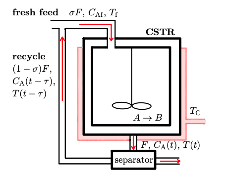
Continuous Stirred-Tank Reactor, or CSTR, is a commonly used model of a chemical reactor, used for mixing reagent in the system. The model is idealized, assuming perfect mixing of reagent within the reactor and that the output composition is identical to the internal composition. Using model with recycle stream [2] and parameters from MATLAB CSTR model [1], the system can be described through set of differential equations as: \[ \frac{d C_\mathrm{A}(t)}{ dt} = \frac{\sigma F}{V} C_\mathrm{Af} (t) - \frac{F}{V} C_\mathrm{A} (t) + \frac{(1 - \sigma)F}{V}C_\mathrm{A} (t - \tau) - r(t) \] \[ \frac{dT(t)}{dt} = \frac{\sigma F}{V}T_\mathrm{f} (t) - \frac{F}{V}T(t) + \frac{(1-\sigma)F}{V} T (t - \tau) - \frac{\Delta H}{\rho C_\mathrm{p}} r(t) - \frac{UA}{\rho C_\mathrm{p} V} (T(t) - T_\mathrm{C} (t)) \] for \[ r(t) = k_\mathrm{0} e ^{-\frac{E}{RT(t)}}C_\mathrm{A} (t) \] The parameters are shown below. The diagram shows the system where an inlet feed stream with temperature \( T_{\mathrm{f}} \) [K] and concentration \( C_{\mathrm{Af}} \) [\( \mathrm{kmol/m^{3}} \)] enters the reactor, where it is continuously mixed. These variables can be adjusted directly by the user and are therefore defined as system inputs. The reactor temperature is also influenced by the coolant jacket temperature \( T_{\mathrm{C}} \) [K], which is likewise defined as an input. The reactor temperature \( T \) [K] and the concentration of reactant A, \( C_{\mathrm{A}} \) [\( \mathrm{kmol/m^{3}} \)], are assumed to be measurable states of the system.

Parameters	Value	Unit	Description
\( F \)	1	\( \mathrm{m^3/h} \)	Volumetric flow rate
\( V \)	1	\( \mathrm{m^3} \)	Reactor volume
\( R \)	1.985875	\( \frac{\mathrm{kcal}}{\mathrm{kmol \cdot K}} \)	Boltzmann's ideal gas constant
\( \Delta H \)	-5960	\( \frac{\mathrm{kcal}}{\mathrm{kmol}} \)	Heat of reaction per mole
\( E \)	11843	\( \frac{\mathrm{kcal}}{\mathrm{kmol}} \)	Activation energy per mole
\( k_\mathrm{0} \)	34930800	\( \frac{1}{\mathrm{h}} \)	Pre-exponential nonthermal factor
\( \rho C_\mathrm{p} \)	500	\( \frac{\mathrm{kcal}}{\mathrm{m^3 \cdot K}} \)	Density multiplied by heat capacity
\( UA \)	150	\( \frac{\mathrm{kcal}}{\mathrm{K \cdot h}} \)	Heat transfer coefficient-area product
\( \sigma \)	0.8	-	Output feed ratio

Linearization is realized around operating point:

• \( T_\mathrm{f} = 300 \, \mathrm{K} \)
• \( C_\mathrm{Af} = 10 \, \mathrm{kmol/m^3} \)
• \( T_\mathrm{C} = 299 \, \mathrm{K} \)
• \( T = 373 \, \mathrm{K} \)
• \( C_\mathrm{A} = 2 \, \mathrm{kmol/m^3} \)

tdrlocus example

This leads to transfer function describing temperature change inside the reactor with respect to temperature of coolant jacket and inner delay from the recycle stream: \[ H_\mathrm{1, 21} (s) = \frac{1{,}978 s + 9{,}8438 - 0{,}3956 e^{-3s}}{6{,}591 s^2 + 14{,}59 s + 15{,}86 - (2{,}637 s + 2{,}917) e^{- 3 s} + 0{,}2637 e^{-6 s}} \] The root-locus of the system can be plotted by calling:

reg = [-10, 5, 0, 50];
num = "1.978*s+9.8438 - 0.3956*exp(-3*s)";
den = "6.591*s^2 + 14.59*s + 15.86 - (2.637*s + 2.917)*exp(-3*s) + 0.2637*exp(-6*s)";
tdrlocus(reg, num, den);

reg = [-10, 5, 0, 50];
num = "1.978*s+9.8438 - 0.3956*exp(-K1*s)";
den = "6.591*s^2 + 14.59*s + 15.86 - (2.637*s + 2.917)*exp(-K1*s) + 0.2637*exp(-2*K1*s)";
tdrlocus(reg, num, den);

reg = [-10, 5, 0, 50];
num = "(1.978*s+9.8438)*exp(-0.1*K2*s) - 0.3956*exp(-(K1+0.1*K2)*s)";
den = "6.591*s^2 + 14.59*s + 15.86 - (2.637*s + 2.917)*exp(-K1*s) + 0.2637*exp(-2*K1*s)";
tdrlocus(reg, num, den);